Live UFC Analytics Platform
Live Scoring Model:
See how real-time stats fuel live score predictions and win probabilities through a streamlined modeling process.
Live Data Collection:
A Python script I wrote scrapes ESPN Fightcenter at the end of each round. The script collects:
- Total strikes landed
- Significant strikes (broken up by target)
- Control time
- Takedowns
- Submission attempts
Below is an example of what the ESPN stat feed looks like at the end of a round:
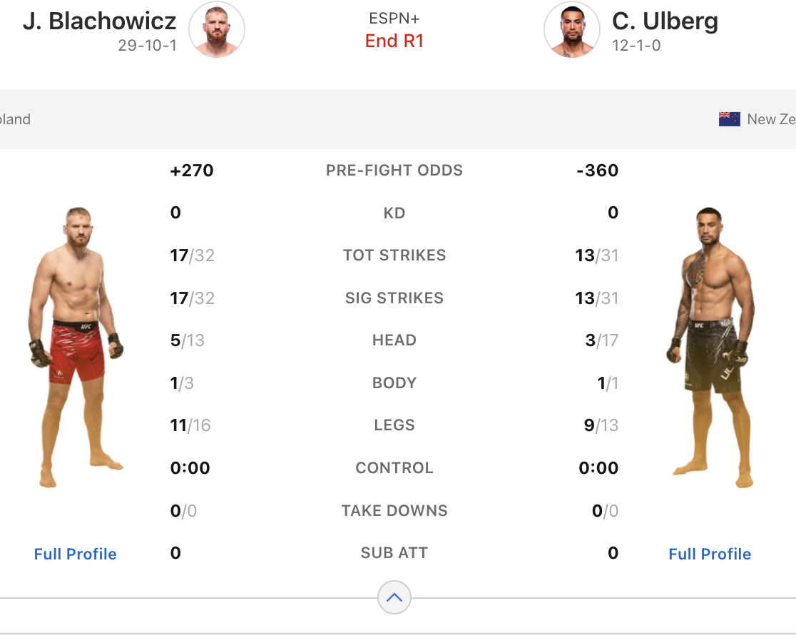
Stat differences are calculated from the red corner’s perspective and used to estimate round win probabilities. For the round above (Błachowicz was red), the differences are:
- 2 Significant Head Strikes (5 - 3)
- 0 Significant Body Strikes (1 - 1)
- 2 Significat Leg Strikes (11 - 9)
No other stats were recorded, so the model only used the differences in head & leg strikes here.
The Model:
To eliminate bias, fighters were first randomly assigned to either column in the dataset. For each round, the difference in fight statistics between the two fighters was calculated.
The response variable was structured as a four-level factor representing possible round outcomes:
- 10-8 for Fighter 1
- 10-9 for Fighter 1
- 10-9 for Fighter 2
- 10-8 for Fighter 2
This setup allows the model to capture both the direction and the margin of victory in each round.
The scoring model I built is an ordered logistic regression model (ordered GLM). It takes the stat differences as input and returns the predicted probability of each of the four outcomes. The total win probability for each fighter is also calculated as the sum of their 10-9 win and 10-8 win probabilities.
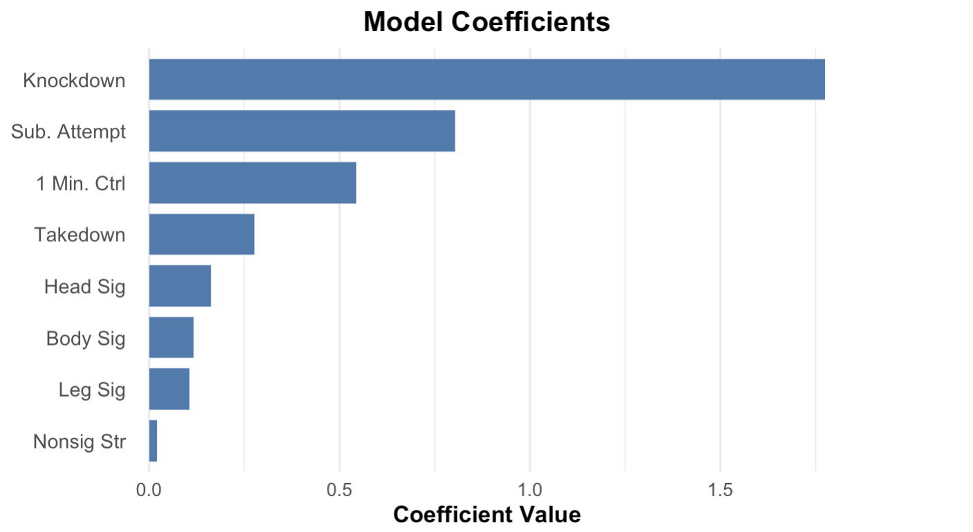
The following graph shows the coeficcient (or value) for each statistic in the model:
Scoring Output:
Utilizing the predicted probabilities, the python script can tweet the predicted winner and score of each round. Depending on the 10-8 probabilities, there are the different scoring messages:
Standard 10-9 (10-8 probability less than 25%):
Round 2 Scoring Model Prediction:
— KO Trends (@KOTrends) March 22, 2025
10-9 Carlos Ulberg
📊61% Win Probability#UFCLondon
10-8 Warning (10-8 probability between 25% and 50%):
Round 2 Scoring Model Prediction:
— KO Trends (@KOTrends) March 9, 2025
10-9 Justin Gaethje
⚠️ Possible 10-8 Round (26% Probability)#UFC #UFC313
10-8 Round (10-8 probability greater than 50%):
Round 1 Scoring Model Prediction:
— KO Trends (@KOTrends) April 6, 2025
10-8 Rhys McKee
🚨 Model predicted a 91% chance of a 10-8#UFC #UFCVegas105
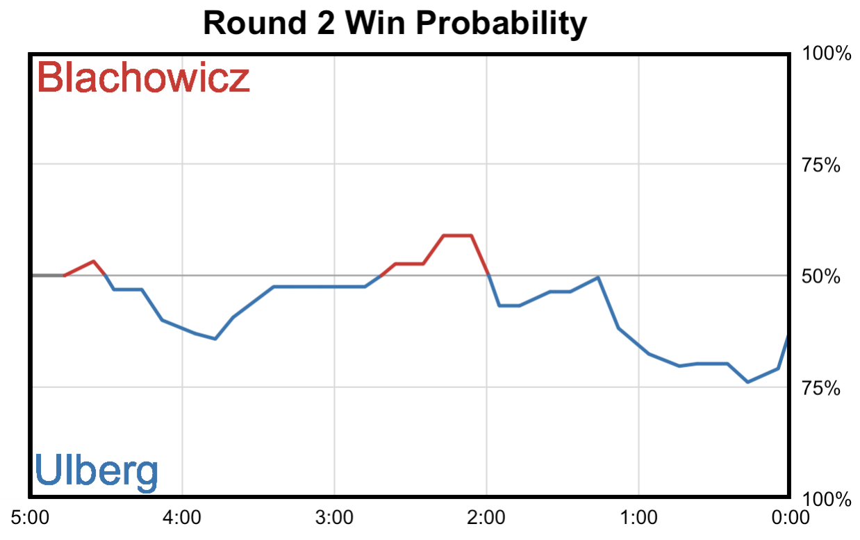
Live Win Probability Graphs:
Using additional code to scrape ESPN Fightcenter during rounds, I can collect live data whenever it updates. This live data refreshes about every 10 seconds, and using the same model framework discussed above I can predict the win probability for each fighter at any point during the round.
Win probability graph Example:
Fighter Performance Ratings Formula:
The UFC rankings are a key part of the sport’s ecosystem, but as with any system influenced by human voting they can be shaped by perception and promotional dynamics. To offer an alternative lens, I created an objective rankings model that evaluates fighters purely on results and quantifies fighter stock in a consistent, data-driven way.
Explore The Rankings:
Use the interactive tool below to browse my updated rankings:
My Rankings Formula Explained:
This formula was originally designed based off of ELO skill ratings used in chess. After each game, a player’s rating goes up or down depending on the opponent’s rating. Beating a higher-rated player than you gives a bigger ELO boost, while losing to a player rated lower than you causes a bigger drop.
I started by applying the classic ELO rating system to UFC fights, which provided a solid foundation. From there, I modified the formula to account for factors that reflect the quality of a victory (such as early finishes and title fights) and added a decay function to account for inactivity. Once the final structure was in place I ran a grid search to tune key parameters like rating sensitivity and decay rate, optimizing the model’s prediction accuracy.
Post-Fight Adjustment Formula:
The formula I have created goes through all UFC Fights since UFC 17 in chronological order, and adjusts both fighters’ ratings after each fight. For a fighter’s first fight in the UFC, they are given a default rating of 300. For each fight in the data, the model calculates the expected win probability using the following formulas for the winner and loser:
WinProbW = 1 / (1 + 10 (RatingL - RatingW) / 370)
WinProbL = 1 / (1 + 10 (RatingW - RatingL) / 370)
The expected win probabilities are then used in these formulas to calculate the new fighter ratings:
NewRatingW = RatingW + 170 × Title × Method × (1 - WinProbW) × (1 + RatingL⁄40000)
NewRatingL = RatingL - 170 × Method × (-1 + WinProbL) × (1 - RatingW⁄40000)
To account for the added significance of title fights, the variable Title applies a 5% bonus to the winner’s rating change after title wins.
The Method variable adjusts the rating impact based on how the fight was won or lost. A first-round finish sets Method = 1.5, giving a 50% boost to the rating change, while a standard three-round decision results in Method = 1.0. For split decisions, Method = 0.9 to reflect the uncertainty of the outcome.
The (1 - WinProb) part of the formula is the ELO system explained earlier, so it will scale the changes in ratings based on differences in pre-fight ratings (larger changes for bigger rating gaps).
The final part of the formula (1 - RatingW⁄40000) gives bigger boosts for beating strong opponents and smaller penalties for losing to them. It doesn’t look at the rating difference, but instead scales by the opponent’s overall strength. So beating an elite fighter means more than beating someone average, and losing to a top fighter hurts less because of this part.
Rating Decay:
While the formula above does a good job of capturing fighter merit, it does not account for long periods of inactivity. To address this, a decay function was added to penalize inactivity and gradually remove inactive fighters from the rankings.
Rating decay begins 270 days (approximately 9 months) after a fighter’s most recent bout. At that point, their rating is reduced by 3%. Once on the decay clock, a fighter’s rating continues to decrease by an additional 3% every 90 days of further inactivity. The decay clock is fully reset whenever the fighter competes again, regardless of outcome.
Future Implementations:
While this model provides a strong foundation for ranking fighters, there are still several areas I plan to improve. The next addition I’m exploring is incorporating weight class adjustments.
The main challenge is that changing weight classes isn’t always a disadvantage; fighters may move up or down and still perform at a high level. Because of this, I’m considering applying weight class adjustments only in rare cases, such as champion vs. champion matchups, where the implications of weight differences are most significant.
On a larger scale, one of the model’s current limitations is the lack of ratings for a fighter’s UFC debut due to data limitations. However, I’m currently working on scraping fight records from before a fighter’s UFC career. With this expanded dataset, the model could not only provide more accurate debut ratings but also potentially scale beyond the UFC, allowing for a more comprehensive global ranking system.
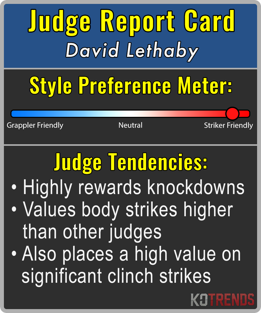
Judge Report Cards:
My judge report cards are designed to showcase the stylistic preferences of UFC judges. Utilizing the models I created in my Senior Thesis Project, I am able to identify which fight statistics most correlate with an individual judge’ scorecards. Additionally, I created a metric that I call striker-grappler preference score (sgps) to better quantify a UFC judges’ stylistic preferences.
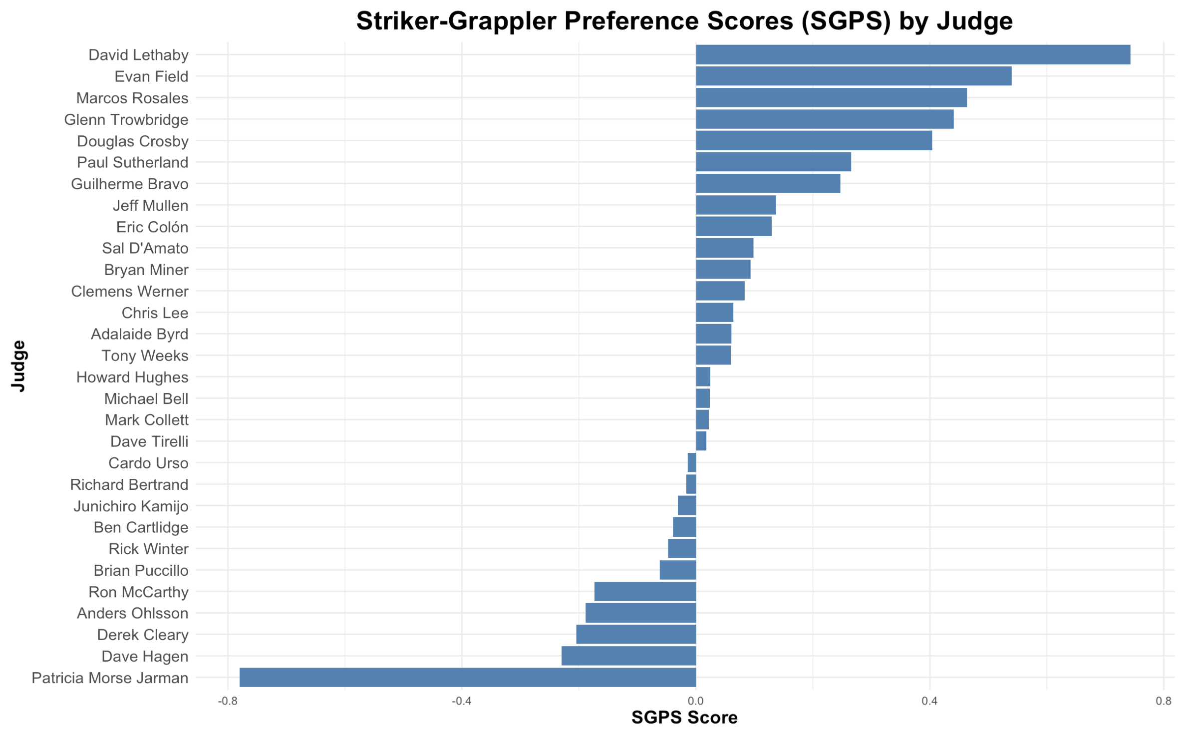
Striker-Grappler Preference Scores (SGPS):
In order to create a single metric that identifies a judges’ stylistic preference, one of the models from my Senior Thesis was used. The predictors were first broken into the following categories:
Striking predictors:
- Significant distance strikes
- Significant clinch strikes
- Knockdowns
Grappling predictors:
- Significant ground strikes
- Takedowns
- Control time
- Submission attempts
- Reversals
Then, using the judge & non-judge models from My Thesis, I repeated this process for each judge:
- 4 values were first calculated:
- strj = sum of the judge model striking coeficcients
- graj = sum of the judge model grappling coeficcients
- strnj = sum of the non-judge model striking coeficcients
- granj = sum of the non-judge model grappling coeficcients
- These were then used to calculate ratiostr and ratiogra
- ratiostr = strj/strnj
- ratiogra = graj/granj
- Ratios are used to calculate scores for each judge (higher numbers prefer strikers):
- SGPS = log(ratiostr/ratiogra)
Positive SGPS values indicate a preference for striking, while negative values reflect a preference for grappling. The chart below displays the SGPS scores for the 30 UFC judges with the most rounds judged:
Final Report Cards:
The striker-grappler preference scores provide the main output for these judge report cards. I can then utilize the models to identify specific scoring preferences of individual judges. These are periodically posted throughout events, as well as at the start of the main event after the three judges are accounced. Some examples of these report cards are showcased below: